CHAPTER 18
Surface codes and decoding
Learning goals. Read a surface-code patch, calculate syndromes, distinguish data and measurement errors, and interpret distance scaling with the correct noise model.
18.1 Local checks encode nonlocal information
Surface codes arrange data qubits and local X- and Z-type parity checks on a two-dimensional layout. Neighboring checks overlap on an even number of data qubits, so they commute. Error strings create changes in nearby checks; logical operators connect appropriate boundaries or wrap nontrivially around the surface [37, 38].
A rotated planar distance-d patch with one measurement ancilla per independent check has d² data qubits and d²−1 syndrome ancillas, totaling . Extra qubits may be needed for leakage removal, routing, surgery, or spare capacity. This expression is a memory-patch count, not the physical size of an entire useful logical computer.
18.2 A complete distance-three example
Number the nine data qubits row by row, 0–2 on top, 3–5 in the middle, 6–8 on the bottom. The following eight independent commuting generators define the patch used in the laboratory:
| Check | Data-qubit Pauli product |
|---|---|
| X0 | |
| X1 | |
| X2 | |
| X3 | |
| Z0 | |
| Z1 | |
| Z2 | |
| Z3 |
There are n=9 data qubits and r=8 independent checks, so k=1. Representatives of logical operators are
They commute with every check, anticommute with each other at their one shared location, and have weight three. No weight-one or weight-two nontrivial logical Pauli exists for this code, so its distance is three.
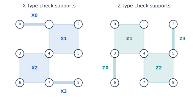
Worked syndrome. An X error on the center data qubit 4 anticommutes with Z1 and Z2 and commutes with the remaining checks. A Z error on 4 anticommutes with X1 and X2. A Y error has both effects. The syndrome contains information about violated parity constraints, not the logical α and β.
18.3 A syndrome does not identify a unique error
If E and E’ differ by a stabilizer, they act identically on the code space and have the same syndrome. If they differ by a nontrivial logical operator, they also have the same syndrome but act differently on the logical information.
A decoder chooses a recovery R based on the syndrome and noise model. Success requires RE to be a stabilizer (up to phase). Requiring R=E is unnecessarily strict because stabilizer-equivalent corrections are equally successful. A zero residual syndrome alone is insufficient: an undetected logical operator also has zero syndrome.
The laboratory uses a minimum-weight Pauli recovery for this fixed patch with perfect measurements and equal costs for X,Y,Z. This is a code-capacity teaching model. It is not a full circuit-level surface-code decoder or a maximum-likelihood decoder accounting for degeneracy.
Laboratory L24 — Surface-code syndromes. Click data qubits to cycle through I,X,Y,Z errors. Inspect all eight checks, the chosen minimum-weight recovery, and the residual logical action. Try a full logical string and observe its zero syndrome.
18.4 Noisy checks require time as well as space
In a physical processor, a stabilizer measurement uses several gates and an ancilla that can itself fail. A wrong readout can mimic a data error. Repeating checks lets a decoder distinguish persistent spatial changes from isolated temporal changes.
A detector often compares check outcomes across consecutive rounds. Decoding graphs then have both spatial and temporal edges. A chain of data and measurement faults can connect boundaries in spacetime and cause logical failure. Minimum-weight perfect matching is one important decoding approach; correlated decoders, belief propagation, and learning-based methods address other models or structures [39].
The syndrome circuit’s gate order matters. An ancilla fault can propagate to multiple data qubits as a hook error. Scheduling must preserve the intended effective distance. A stabilizer table alone does not specify a fault-tolerant extraction circuit.
18.5 Thresholds are properties of complete protocols
Below a suitable physical-noise threshold, increasing code distance can reduce logical error. A common illustrative scaling form is
Here p summarizes a specified noise model, depends on the code, circuit, and decoder, and A is fitted or modeled. This is not a universal exact law. Different physical error types, biased noise, correlations, leakage, and finite-size effects can change it.
If , increasing d by two reduces the model’s pL by ten. If , the same expression increases instead; extrapolating a favorable below-threshold trend into that regime is invalid.
Google’s Willow work reported distance scaling below threshold for surface-code memories, with a distance-seven logical error per cycle of approximately 0.143% and a suppression factor about 2.14 when increasing distance by two [47]. The reported experiment used additional hardware beyond the bare patch and particular decoding methods. Its scope is a memory demonstration, not a completed universal large-scale computation. The 2026 correction notice and publication dates are recorded in Chapter 24.
18.6 Measuring progress toward a logical machine
Useful reports specify code distance, data and ancillary qubits, number of rounds, state bases, decoder, acceptance fraction, error bars, and failure metric. “Logical qubit” can refer to an encoded state, an error-detected state, a repeatedly corrected memory, or a subsystem supporting logical operations. These achievements should not be ranked by a single unqualified logical-qubit count.
A real-time decoder also needs adequate throughput and manageable response latency. A stream can have high throughput while each answer arrives several cycles later. Some operations tolerate delayed Pauli-frame updates; others require a timely classical decision. This motivates the architecture discussion in Chapter 19.
18.7 Exercises
18.1. Find the syndrome of in the patch.
Show solution / guidance
It anticommutes only with Z1. All X checks commute with it, and the other Z supports exclude qubit 0.
18.2. Why does have zero syndrome?
Show solution / guidance
It overlaps Z0 on two qubits and Z1 on two, and the other Z checks on zero. All overlaps are even; X checks commute automatically.
18.3. Count bare data and syndrome qubits for d=5.
Show solution / guidance
25 data plus 24 syndrome ancillas equals 49 physical qubits. Additional architecture overhead is outside this count.
18.4. For A=0.1,p/pth=0.1, compare d=3 and d=7 in the illustrative model.
Show solution / guidance
gives ; d=7 gives . The two distance increments each supply a factor ten.
18.5. Does “all stabilizers +1 after recovery” prove success?
Show solution / guidance
No. The residual may be a logical Pauli with zero syndrome. Compare the residual’s logical commutation or an appropriate logical measurement.